pvigier's blog
computer science, programming and other ideas
Pychain Part 1 - Computational Graphs
Welcome in this big tutorial on neural networks!
Our goal is to write our own deep learning framework like TensorFlow or Torch. We are going to learn in-depth how neural networks work, all the mechanics behind them.
We will get our hands dirty and code everything! In this tutorial, we will use Python3 and scipy but I hope that the code and the ideas are clear enough so that you can adapt the code to your favorite language.
First, I show you the plan. In this part, we are going to quickly introduce neural networks and then, we will introduce computational graphs in order to model them. In the end of this part, we are going to use our implementation to learn some non-linear functions.
In the second part, we will deal with a more serious problem. We are going to build an optical character recognition system upon the MNIST database. It is a classical problem in machine learning, we have to do it.
Then, we will tackle recurrent neural networks and show how to model them with our library. To apply our new knowledge, we will try to learn a formal grammar generated by an automaton.
In part 4, we will go further with recurrent neural networks and introduce the well-known LSTM cell. We will briefly compare it with fully-connected recurrent neural networks.
To approach part 6, some more efficient optimization algorithms are necessary. Consequently, we will discuss them in part 5.
Have you ever read this fabulous article by Andrej Karpathy? Yes? Cool, because, we are going to reproduce his results with our own library in part 6. Amazing, isn’t it?
Finally, parts 7 and 8 are going to be theoretical appendices for the most curious readers.
Is it all? Maybe not! Stay tuned!
If you are ready, let’s go!
Neural Networks
I am not going to make a long presentation on neural networks. Why? Because there are already a lot of good pages on the web about them.
If you want a gentle introduction to them, you can read these pages by Michael Nielsen. It is well written and easy to follow.
If you want a more academic and in-depth text on neural networks, I must advise you to read the amazing Deep Learning Book (aka The book). I learnt a lot from this book. Lots of ideas that I will present in this tutorial are inspired by it.
During the redaction of these articles, I discovered this course from Stanford. I encourage you to have a look on it!
Another reason why I do not present neural networks, is that we will adopt a modern approach on them. We are not going to see a neural network as a network of neurons but instead we will consider it as a parametric function.
Machine Learning
The Learning Problem
Let’s speak a bit of machine learning, more precisely of supervised learning. In supervised learning, there is an unknown function \(g : \mathcal{X} \rightarrow \mathcal{Y}\) and we have a dataset of examples \(D = ((x_1, y_1), ..., (x_N, y_N))\) such that \(\forall (x, y) \in D, y = g(x)\). The goal is to use the dataset \(D\) to reconstruct \(g\). In other words, we want to find a function \(f\) such that:
\[\forall x \in \mathcal{X}, f(x) \approx g(x)\]To go further we have two issues to tackle. The first one is that we have not access to the value of \(g\) for all \(x\) in \(\mathcal{X}\), only those in \(D\). Consequently, we will use a method called empirical risk minimization (ERM). Intuitively, we will try to have \(\forall (x, y) \in D, y \approx f(x)\) and hope that it works well for the other values.
Then we need to formalize a bit the approximation symbol \(\approx\). To do that, we will use a cost function, we will note it \(J\). There are a variety of different cost functions, a famous one is the quadratic cost:
\[J(f, D) = \sum_{(x, y) \in D}{||y - f(x)||_2^2}\]If you want to know more about cost functions, how to derive them from statistics, regularization, etc. You are welcome to read the appendix on cost functions.
Now that we have a cost function, our goal is to find a function \(f\) such that \(J(f, D)\) is small.
We still have a big problem. What is \(f\)? We could try to find the best \(f\) in the whole space of functions but it is not a good idea because there is an infinity of functions which have a cost equal to zero and most of them generalize very badly. We will instead restrict ourselves to a specific class of smoother functions and for that we are going to use, like I said before, parametric functions. A parametric function is simply a function \(f_{\theta}\) that depends on a parameter \(\theta\).
The problem is now to find the best possible \(\theta\) to fit our data. Formally, we will try to solve the following problem:
\[\theta^* = \underset{\theta}{argmin}J(f_{\theta}, D))\]Such a problem is called an optimization problem and there exist good tools to tackle it.
Gradient Descent
I am going to quickly present an algorithm to find a good \(\theta\). The algorithm is called gradient descent. It consists of choosing randomly an initial parameter \(\theta_0\) and at each step of the algorithm we will optimize locally to improve the solution. The idea is to make small steps to diminish the cost. We have to decide in which direction we make these steps.
Thanks to Taylor’s theorem, we know that around a point \(x_0\), a differentiable function \(f\) can be approximated by:
\[f(x) \approx f(x_0) + \frac{\partial f}{\partial x}(x_0)^T(x - x_0)\]Maybe you are more familiar with the 1D case which says that around a point a differentiable function can be approximated by its tangent:
\[f(x) \approx f(x_0) + f'(x_0)(x - x_0)\]Let’s visualize what this formula means and how it can be useful to find a good direction. The generalization of the tangent, which is a line, in a vector space is a hyperplane. In a 2D space it corresponds to a plane.
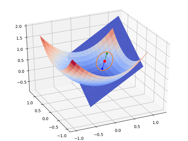
The plane in blue is the approximation given by Taylor’s theorem. The points in orange are the outputs of \(f\) for all points at a same distance \(d\) to \(x_0\). In green, it’s the output of the point at distance \(d\) of \(x_0\) in the direction of the gradient and in blue, it’s the output of the point at distance $d$ in the opposite direction of the gradient.
You can clearly see that the direction toward which the plane goes up the quickest is the gradient \(\frac{\partial f}{\partial x}(x_0)\). Conversely, the direction in which it goes down the quickest is the opposite of the gradient \(-\frac{\partial f}{\partial x}(x_0)\).
If you are more a math person who likes to play with formulas, you can remark that \(\frac{\partial f}{\partial x}(x_0)^T(x - x_0)\) is an inner product. And, if we consider all points at the same distance \(d\) to \(x_0\), the Cauchy-Schwarz inequality tells us that this term is maximized when the point \((x - x_0)\) has the same direction as the gradient and is minimized when the point has the opposite direction of the gradient.
Let’s go back to our goal to minimize the cost. Let \(\theta_t\) be the value of the parameter at iteration \(t\) of the algorithm. We can see \(J\) as a function of \(\theta\), and we want to find a point around \(\theta_t\) that has a lower cost. Using our first order approximation of \(J\) around \(\theta_t\) we know that the direction toward which the cost is decreasing the most is \(-\frac{\partial J}{\partial \theta}(\theta_t)\). Consequently, we will make a small step in this direction and choose the point:
\[\theta_{t+1} = \theta_t - \eta \frac{\partial J}{\partial \theta}(\theta_t)\]where \(\eta\) is called the learning rate. It is a parameter that controls the size of the steps we make. We will dig deeper into optimization algorithms later in another part.
You can see gradient descent in action, in the animation below.
You can get the code of these two simulations here.
I stop there for the brief introduction to machine learning. We will now see how to model some parametric functions and how they relate to neural networks.
Computational Graphs
A computational graph is a graph which represents a computation.
Let’s see some examples to show how this tool can be used to model useful functions.
Imagine, you want to fit very simple data like in the figure below.
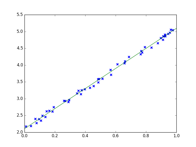
The natural idea is to use a function like this one \(f_{\theta} : x \mapsto ax + b\) where \(\theta = (a, b)\) is the parameter of the function. This function can be represented with the following computational graph.

Now, imagine you have to solve a more difficult problem and you want to use a neural network, like the one below.

It has two layers, the hidden layer uses \(\tanh\) as activation function and the output layer uses the sigmoid \(\sigma : t \mapsto \frac{1}{1 + \exp(-t)}\).
This model is strictly equivalent to the function \(f_{\theta} : x \mapsto \sigma(\tanh(xW_1)W_2)\) where \(W_1\) are the weights of the first layer and \(W_2\) the weights of the second layer. In this case again, \(f\) is a parametric function which depends on \(\theta = (W_1, W_2)\).
The following computational graph corresponds to the neural network depicted above.

We can see several things from these examples. Firstly there are different nodes:
- Input nodes (in rose): they represent the inputs of the function. In our examples, they are the \(x\) nodes.
- Operation nodes (in blue): they are nodes that represent operations. They take inputs, make a computation and give ouputs. In our examples, the \(\sigma\), \(\tanh\), \(\times\), \(+\) nodes are operation nodes.
- Parameter nodes (in green): they represent the parameters of the function. In our example, they are \(a\), \(b\), \(W_1\) and \(W_2\).
Secondly, it allows a more compact notation, instead of drawing lots of neurons, we can only draw few nodes to represent a whole network.
Finally, we can model a broader class of parametric functions. We are not limited at all by the biological inspiration. You can unleash your engineering spirit and craft all sort of functions.
In the next sections, we will explain how to code a computational graph to model a parametric function and how to optimize them to fit your data.
Architecture of the Library
First, I am going to present the architecture of the library. Then we are going to explain the code.
There are three main classes that we are going to code in this part: the Node class, the Graph class and the OptimizationAlgorithm class.
The Node class contains most of the logic of the library. It’s the hard part.
The Graph class is a container that contains nodes and allows to interact easily with them.
Finally, the OptimizationAlgorithm class implements an optimization algorithm like the gradient descent algorithm we have described above. The class uses the parameter nodes and optimizes their value to minimize the cost. This class will allow us to easily switch between different algorithms. If you are familiar with design patterns, you should have recognized the strategy pattern.
The UML diagram below gives a global view of the classes and their interactions.

And before, I forget you can retrieve the full code for this chapter here.
Node Class
A node have several inputs and several outputs. During the propagation, a node uses its inputs to compute its ouputs as depicted below.

The goal of the backpropagation is to compute the derivative of the cost with respect to the parameters to use the gradient descent algorithm. To do that, we are going to use the chain rule, a lot. Indeed, thanks to the chain rule, it is possible to express the derivative of the cost with respect to an input of a node with the derivatives of the cost with respect to the outputs of the same node.

Precisely, if a node has \(m\) inputs and \(n\) outputs, we have:
\[\forall i \in \{1, ..., m\}, \frac{\partial J}{\partial x_i} = \sum_{j=1}^{n}{\frac{\partial y_j}{\partial x_i}\frac{\partial J}{\partial y_j}}\]And the term \(\frac{\partial y_j}{\partial x_i}\) only depends of the nature of the node.
Consequently, we are going to backpropagate the derivatives from the “end” of the graph to the parameter nodes.
An illustration with the neural networks shown before:

Base Class
Most of the code is contained in the base class. We are going to divide the work in two stages. First, we are going to see the methods that are useful to create the computational graph. Then we are going to describe the methods used during the propagation and the backpropagation.
Let’s see the first part of the code.
class Node:
    def __init__(self, parents=None, nb_outputs=1):
        # Parents for each input
        self.set_parents(parents or [])
        # Children for each output
        self.children = [[] for _ in range(nb_outputs)]

        # Memoization
        self.x = None
        self.y = None
        self.dJdx = None
        self.dJdy = None

        # Dirty flags
        self.output_dirty = True
        self.gradient_dirty = True

    def set_parents(self, parents):
        # Fill self.parents
        self.parents = []
        for i_input, (parent, i_parent_output) in enumerate(parents):
            self.parents.append((parent, i_parent_output))
            parent.add_child(self, i_input, i_parent_output)

    def add_child(self, child, i_child_input, i_output):
        self.children[i_output].append((child, i_child_input))
A node has a list of its parents, the list have the following form [(node1, i_output1), (node2, i_output2), ... ]. For each parent node, we precise the index of its output to which the current node is connected. The first couple corresponds to the first input of the node \(x_1\), the second to \(x_2\), etc.
A node has a 2D list of its children too. The first dimension is the output index. And for each output index, there is a list containing the nodes connected to this output. The list has the following form [(node1, i_input1), (node2, i_input2), ...]. For each child node, we precise the index of its input that is connected to this output.
OK, it is a bit hard to follow. Hopefully, a diagram will make it crystal clear!

We can set the parents during the initialization or later by using set_parents. We have not to manually set the children.
That’s all for the dependencies between nodes.
class Node:
   # ...

   def get_output(self, i_output):
        if self.output_dirty:
            self.x = [parent.get_output(i_parent_output) \
                for (parent, i_parent_output) in self.parents]
            self.y = self.compute_output()
            self.output_dirty = False
        return self.y[i_output]

    def compute_output(self):
        raise NotImplementedError()

    def get_gradient(self, i_input):
        # If there are no children, return zero
        if np.sum(len(children) for children in self.children) == 0:
            return np.zeros(self.x[i_input].shape)
        # Get gradient with respect to the i_inputth input
        if self.gradient_dirty:
            self.dJdy = [np.sum(child.get_gradient(i) \
                for child, i in children) for children in self.children]
            self.dJdx = self.compute_gradient()
            self.gradient_dirty = False
        return self.dJdx[i_input]

    def compute_gradient(self):
        raise NotImplementedError()

    def reset_memoization(self):
        # Reset flags
        self.output_dirty = True
        self.gradient_dirty = True
The implementation of propagation and backpropagation is very symmetrical.
The method get_output asks the parents of the node their outputs and save them in self.x. Then we use, compute_output and we save the result in self.y. Finally, we set the dirty flag to false. We use memoization not to compute twice the same value. It is very important because each child will ask the node for outputs, and recursively this node will ask its parents for their outputs, etc. If we do not use memoization, we would waste a lot of time doing unnecessary computations.
The method compute_output is abstract, it will be implemented in specialized classes.
get_gradient is very similar to get_output, for each output we gather the derivative of the cost with respect to this output and save it in self.dJdy. Then we use compute_gradient to compute self.dJdx and set the dirty flag to false.
Finally, there is the method reset_memoization to set the flags to true.
In the next subsections, we are going to see the specializations of this class.
Input Nodes
The class InputNode has an attribute value that can be set. The function get_output is overloaded to directly return this value.
class InputNode(Node):
    def __init__(self, value=None):
        Node.__init__(self)
        self.value = value

    def set_value(self, value):
        self.value = value

    def get_output(self, i_output):
        return self.value

    def compute_gradient(self):
        return [self.dJdy[0]]
Parameter Nodes
The class ParameterNode has a new parameter w. We use the letter w to refer to the weights, like in neural networks.
The output of the node is simply the weight.
class ParameterNode(Node):
    def __init__(self, w):
        Node.__init__(self)
        self.w = w

    def compute_output(self):
        return [self.w]

    def compute_gradient(self):
        return [self.dJdy[0]]
This class is very simple. The only issue is that the constructor expects an initial value for the weights. There are several thumb rules regarding the initialization of the weights. The general idea is to sample from a zero mean distribution with a small standard deviation. You can see more details about initialization in Efficient BackProp.
You will see several examples of initialization later in the tutorial.
Operation Nodes
Then there are the operation nodes. There is a lot of implemented nodes, I am not going to describe the code for each of them.
Let’s take the example of the SigmoidNode which implements the function \(\sigma\) element-wise applied.
We only plug the formulas for the output and the gradient in the methods get_output and get_gradient.
class SigmoidNode(Node):
    def compute_output(self):
        return [1 / (1 + np.exp(-self.x[0]))]

    def compute_gradient(self):
        return [self.dJdy[0] * (self.y[0]*(1 - self.y[0]))]
To have decent performances in Python, it is very important to use numpy at most and to forbid for-loops. Consequently, it is important to express the formulas in term of matrix operations.
If you want to see all the formulas and how to derive the backpropagation formulas, you can go to the appendix on matrix derivations.
Gradient Nodes
The last type of node is the GradientNode. I have never spoken about gradient node yet. There are very similar to input nodes but this time, it is the value of the gradient that can be set.
class GradientNode(Node):
    def __init__(self, parents, value=1):
        Node.__init__(self, parents)
        self.value = value

    def set_value(self, value):
        self.value = value

    def compute_output(self):
        return self.x

    def get_gradient(self, i_input):
        return self.value
During backpropagation, if every node asks their children for gradient, to whom the “last” node asks its gradient with respect to its output? Gradient nodes are the answer to this question. We can set the gradient to be backpropagated.
There are two ways of doing this. We can just add a gradient node as a child to the output node of the graph. Then, we set manually the value of the gradient node to the derivative of the cost with respect to the output of the graph.
Another way of proceeding that I prefer is to add the cost function directly in the computational graph. Then, we just have to add a gradient node with a value of \(1\) as a child of the cost node. And that’s it!
Consider the graph representing the neural networks described above. If we had an input node \(y\) to represent the expected output and we choose the squared error as cost function, we obtain this new graph:

The yellow node at the end is a gradient node which always returns 1 as gradient.
Graph Class
The Graph class is very simple.
class Graph:
    def __init__(self, nodes, input_nodes, output_nodes, expected_output_nodes, cost_node, parameter_nodes):
        self.nodes = nodes
        self.input_nodes = input_nodes
        self.output_nodes = output_nodes
        self.expected_output_nodes = expected_output_nodes
        self.cost_node = cost_node
        self.parameter_nodes = parameter_nodes

        # Create a gradient node
        GradientNode([(cost_node, 0)])

    def propagate(self, X):
        self.reset_memoization()
        for x, node in zip(X, self.input_nodes):
            node.set_value(x)
        return [node.get_output(0) for node in self.output_nodes]

    def backpropagate(self, Y):
        for y, node in zip(Y, self.expected_output_nodes):
            node.set_value(y)
        cost = self.cost_node.get_output(0)
        for node in self.parameter_nodes:
            node.get_gradient(0)
        return cost

    def reset_memoization(self):
        for node in self.nodes:
            node.reset_memoization()

    def get_parameter_nodes(self):
        return self.parameter_nodes
It takes the list of all the nodes in the graph. In addition, it needs to know the function of several nodes in the graph: the inputs, the ouputs, the expected outputs and the cost.
There are also two useful functions:
propagate: to compute the outputs of the graph ;backpropagate: to accumulate the gradient of the cost with respect to the parameters.
Finally, the method reset_memoization resets the flags for all the nodes and get_parameter_nodes returns the parameter nodes. The latter method is useful to give to the optimization algorithm the nodes for which it has to optimize the weights.
Optimization Algorithms
The last class we have to write before we can test our library is the OptimizationAlgorithm class.
The class is a generic template for all first-order iterative optimization algorithms such as gradient descent.
For this kind of algorithm at each step \(t\), we compute a direction \(v_t\) toward which we should move the parameter \(\theta_t\). We have:
\[\theta_{t+1} = \theta_t - \eta v_t\]Where \(\eta\) is the learning rate.
class OptimizationAlgorithm:
    def __init__(self, parameter_nodes, learning_rate):
        self.parameter_nodes = parameter_nodes

        # Parameters
        self.learning_rate = learning_rate

    def optimize(self, batch_size=1):
        for i, node in enumerate(self.parameter_nodes):
            direction = self.compute_direction(i, node.get_gradient(0) / batch_size)
            node.w -= self.learning_rate * direction

    def compute_direction(self, i, grad):
        raise NotImplementedError()
For gradient descent as explained before, we simply have \(v_t = \frac{\partial J}{\partial \theta}(\theta_t)\).
class GradientDescent(OptimizationAlgorithm):
    def __init__(self, parameter_nodes, learning_rate):
        OptimizationAlgorithm.__init__(self, parameter_nodes, learning_rate)

    def compute_direction(self, i, grad):
        return grad
Some Examples
Now we have a fully functional library. The last missing piece is to create a computational graph and try it!
We are going to use fully-connected neural networks to learn two functions respectively XOR and a disk.
We will use the function fully_connected which takes as input a list of the sizes of the layers and returns a computational graph which represents such a network.
def create_fully_connected_network(layers):
    nodes = []
    parameter_nodes = []

    # Input
    input_node = InputNode()
    nodes.append(input_node)

    cur_input_node = input_node
    prev_size = 3
    for i, size in enumerate(layers):
        # Create a layer
        bias_node = AddBiasNode([(cur_input_node, 0)])
        parameter_node = ParameterNode(np.random.rand(prev_size, size)*1-0.5)
        prod_node = MultiplicationNode([(bias_node, 0), (parameter_node, 0)])
        # Activation function for hidden layers
        if i+1 < len(layers):
            # Tanh
            activation_node = TanhNode([(prod_node, 0)])
            # Relu
            #activation_node = ReluNode([(prod_node, 0)])
        # Activation function for the output layer
        else:
            activation_node = SigmoidNode([(prod_node, 0)])
        # Save the new nodes
        parameter_nodes.append(parameter_node)
        nodes += [bias_node, parameter_node, prod_node, activation_node]
        cur_input_node = activation_node
        prev_size = size + 1

    # Expected output
    expected_output_node = InputNode()
    # Cost function
    cost_node = BinaryCrossEntropyNode([(expected_output_node, 0), (cur_input_node, 0)])

    nodes += [expected_output_node, cost_node]
    return Graph(nodes, [input_node], [cur_input_node], [expected_output_node], cost_node, parameter_nodes)
The function is a bit long but simple, we simply create nodes and connect them. First, we create an input node. Then, for each layer, we create a bias node, a parameter node, a multiplication node and an activation node. These nodes model the operation \(x \mapsto f((1 \mid x)W)\) where \((1 \mid x)\) denotes the matrix \(x\) to which we have added a column of 1 at the beginning, \(W\) the weights of the parameter node and \(f\) the activation function.
We use two different activation functions: \(\tanh\) and \(\sigma\). \(\tanh\) is used in the hidden layers, it is a nonlinear function which maps \(\mathbb{R}\) to \(]-1, 1[\). It is very important that activation functions are nonlinear otherwise the multilayer neural network is equivalent to a one layer neural network.
We use the sigmoid function as activation function for the output layer because it maps \(\mathbb{R}\) to \(]0,1[\) and consequently the output of the network can be interpreted as a probability, usually \(p(y=1 \mid x)\).
For the cost function, we choose the binary cross entropy. If you want to know more about the output functions and the cost functions, you can read the appendix.
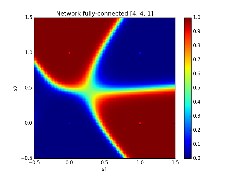
XOR
Learning XOR is an interesting problem because XOR is surely the simplest boolean function that cannot be learnt by a linear classifier. Crafted features or a deep neural network are necessary to solve this nonlinear problem.
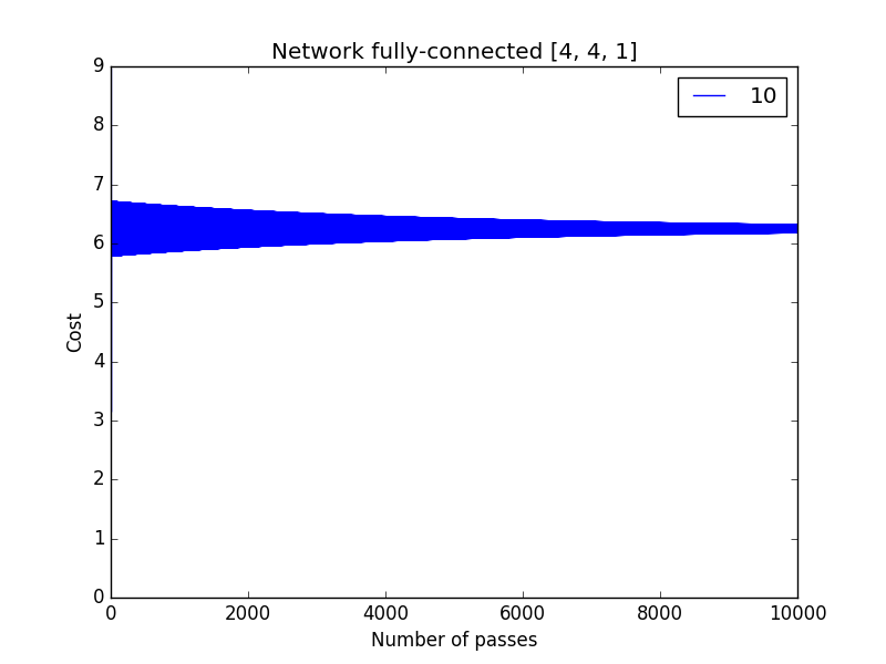
Let’s use this piece of code to train the network.
# Create the graph and initialize the optimization algorithm
layers = [4, 4, 1]
graph = create_fully_connected_network(layers)
sgd = GradientDescent(graph.get_parameter_nodes(), 0.1)
# Train
t = []
costs = []
nb_passes = 10000
for i_pass in range(nb_passes):
    # Propagate, backpropagate and optimize
    graph.propagate([X])
    cost = graph.backpropagate([Y]) / X.shape[0]
    sgd.optimize(X.shape[0])
    # Save the cost
    t.append(i_pass)
    costs.append(cost)
    print(cost)
Finally, you can use the visualize to compute the output of the graph for every \(x \in [-0.5, 1.5]^2\) and see the frontier. You can see that the network models a nonlinear function.
Below, you can see such generated images for two different activation functions for the hidden layers. We can note that \(\tanh\) seems to create smooth frontiers while \(ReLU\) creates sharper ones.
| With tanh | With ReLU |
|---|---|
 |
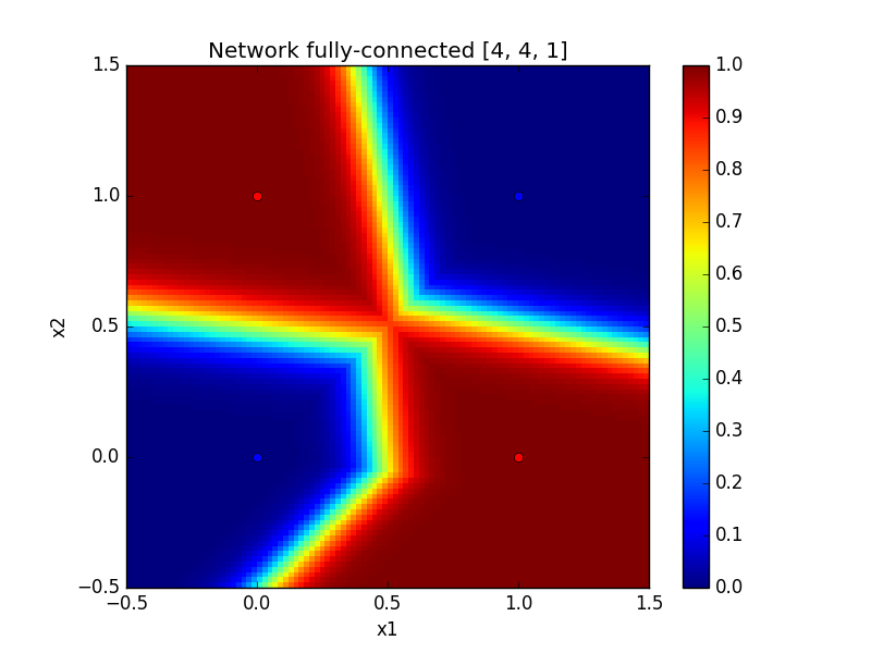 |
Disk
Just for fun let’s learn another function and generate beautiful images. The function we want to learn is such that \(f(x) = 1\) if \(x\) is inside the disk of radius 0.5 and centered on (0.5, 0.5) and \(f(x) = 0\) otherwise.
The function is clearly nonlinear and consequently, it is a perfect problem for a neural network.
To test the code for the disk function, you just have to comment/uncomment few lines in train.py. Below, there are some outputs.
| With tanh | With ReLU |
|---|---|
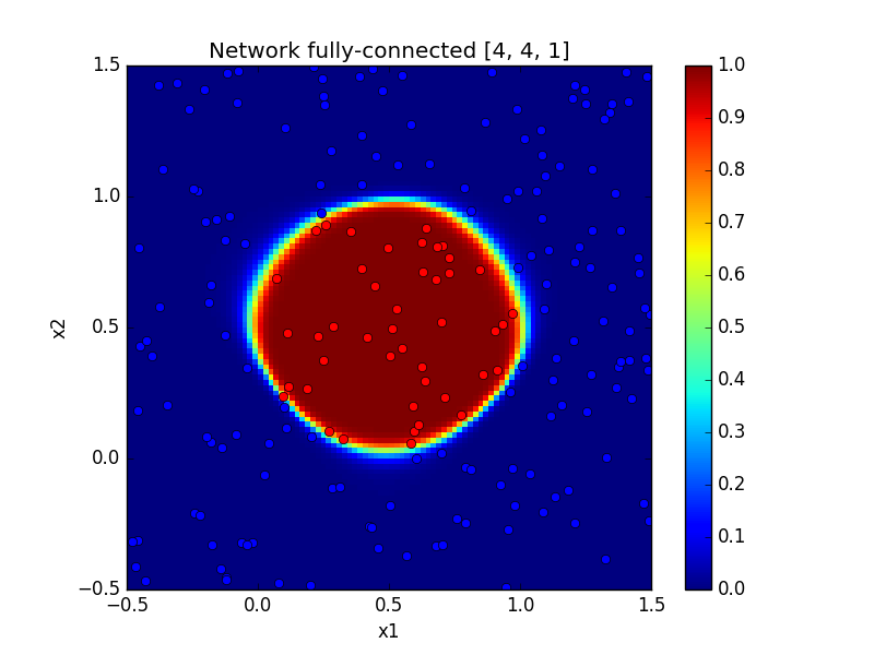 |
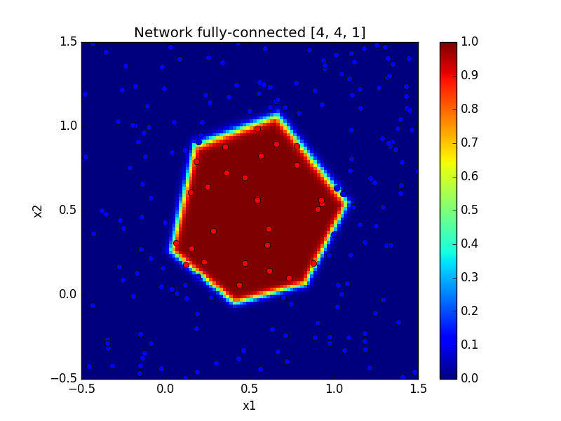 |
To Go Further
Some problems to sharpen your understanding of neural networks:
- What is the smallest number of layers and neurons necessary to perfectly learn the XOR function? Verify your answer by experience. Clues
As mentionned before, one layer (only the output layer) is not sufficient because the frontier would be a straight line. So we should take at least two layers. Each layer should have at least two neurons otherwise the frontier is again a straight line. A network with 2 layers and 2 neurons is the smallest network able to learn the XOR function. You could try to find acceptable weights by hand or you can use gradient descent!
- Study the influence of the learning rate. Clues
Try very small values, values around 1 and very high values.
You can see on the curves below that the cost tends to zero for learning rates small enough. And the larger the learning rate is, the faster the cost tends to zero. However for too large learning rates the cost does not tend to zero anymore.
| Convergence | Divergence |
|---|---|
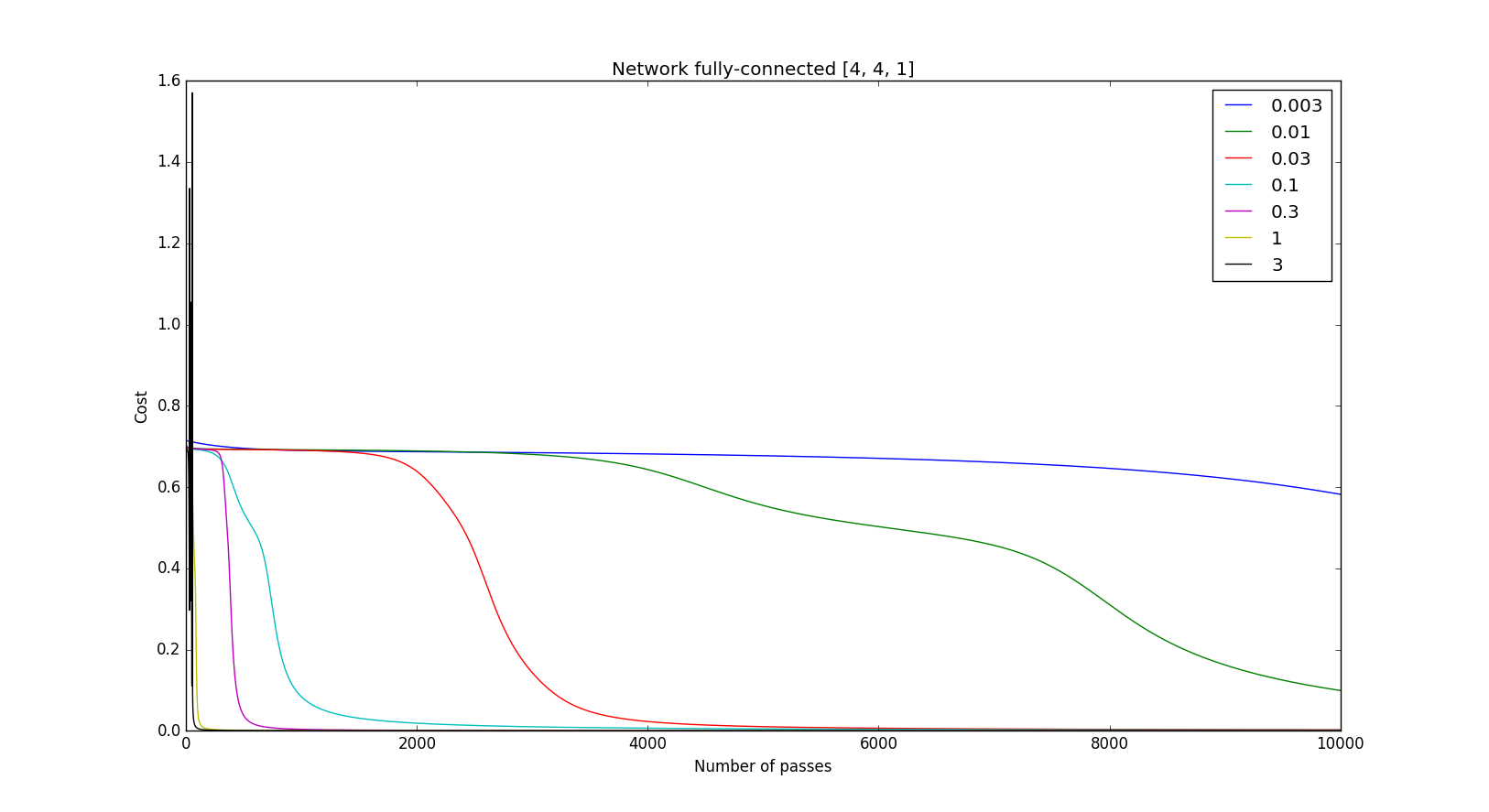 |
 |
- Try to create other datasets using other functions and learn them using a computational graph.
If you are interested in my adventures during the development of Vagabond, you can follow me on Twitter.