pvigier's blog
computer science, programming and other ideas
Fortune's Algorithm: The Details
The last few weeks, I worked on an implementation of the Fortune’s algorithm in C++. This algorithm takes a set of 2D points and construct the Voronoi diagram of these points. If you wonder what is a Voronoi diagram, it looks like this:
For each input point, which is called a site, we want to find the set of points which are nearer to this site than to any other site. These sets of points form cells as you can see on the image above.
What is remarkable about the Fortune’s algorithm is that it constructs such diagrams in \(O(n\log n)\) time (which is optimal for an algorithm which uses comparisons) where \(n\) is the number of sites.
I am writing this article because I find it very hard to implement this algorithm. Until now, it is surely the hardest algorithm I have ever implemented. Thus, I want to share with you the issues I faced and how I solved them.
The code is, as usual, available on github and you will find all the references I used at the bottom of this article.
Fortune’s Algorithm Overview
I will not explain how the algorithm works. Because other people have already done it well. I can recommend you these two blog articles: here and there. The second one is really cool since its author made an interactive demo in Javascript which is useful to understand how the algorithm works. If you want a more formal approach and to see all the proofs, I advise you to read the chapter 7 of Computational Geometry, 3rd edition.
Moreover, I prefer to tackle the implementation details which are not as well documented. And they are what makes this algorithm so hard to implement correctly. I will especially focus on the data structures I used.
I just put a pseudo-code of the algorithm so that we all agree on the global structure of the algorithm:
add a site event in the event queue for each site
while the event queue is not empty
    pop the top event
    if the event is a site event
        insert a new arc in the beachline
        check for new circle events
    else
        create a vertex in the diagram
        remove the shrunk arc from the beachline
        delete invalidated events
        check for new circle events
Diagram Data Structure
The first issue I faced is how to store the Voronoi diagram.
I choose to use a data structure which is widely used in computational geometry called doubly connected edge list (DCEL).
My VoronoiDiagram class has four containers as fields:
class VoronoiDiagram
{
public:
    // ...

private:
    std::vector<Site> mSites;
    std::vector<Face> mFaces;
    std::list<Vertex> mVertices;
    std::list<HalfEdge> mHalfEdges;
}
I will detail each of them.
The Site class represents an input point. Each site has an index, which is useful to query them, coordinates and a pointer to their cell (face):
 struct Site
{
    std::size_t index;
    Vector2 point;
    Face* face;
};
The vertices of the cells are represented by the Vertex class, they just have a coordinates field:
struct Vertex
{
    Vector2 point;
};
Here is the implementation of half-edges:
struct HalfEdge
{
    Vertex* origin;
    Vertex* destination;
    HalfEdge* twin;
    Face* incidentFace;
    HalfEdge* prev;
    HalfEdge* next;
};
You might wonder what is a half-edge. An edge in a Voronoi diagram is shared by two adjacent cells. In the DCEL data structure, we split these edges in two half-edges, one for each cell, and they are linked by the twin pointer. Moreover, a half-edge has an origin vertex and a destination vertex. The incidentFace field points to the face to which the half-edge belongs to. Finally, in DCEL, cells are implemented as a circular doubly linked list of half-edges where adjacent half-edges are linked together. Thus the prev and next fields points to the previous and next half-edges in the cell.
On the image below, you can visualize all these fields for the red half-edge:

Finally, the Face class represents a cell and it just contains a pointer to its site and another to one of its half-edges. It does not matter which half-edge it is because a cell is a closed polygon. Thus we can access to all of its half-edges by traversing the circular linked list.
struct Face
{
    Site* site;
    HalfEdge* outerComponent;
};
Event Queue
The standard way to implement the event queue is to use a priority queue. During the processing of site and circle events we may need to remove circle events from the queue because they are not valid anymore. But most of the standard implementations of priority queues do not allow to remove an element which is not the top one. In particular that is the case for std::priority_queue.
There are two ways to tackle this problem. The first and simplest one is to add a valid flag to events. We set valid to true initially. Then instead of removing the circle event from the queue, we just set its flag to false. Finally, when we process the events in the main loop, if the valid flag of an event equals to false, we simply discard it and process the next one.
The second method which I adopted is not to use std::priority_queue. Instead, I implemented my own priority queue which supports removal of any element it contains. The implementation of such a queue is pretty straightforward. I choose this method because I find it makes the code for the algorithm clearer.
Beachline
The beachline data structure is the tricky part of the algorithm. If not implemented correctly there is no guarantee that the algorithm will run in \(O(n\log n)\). The key to reach this time complexity is to use a self-balancing tree. That’s easier said than done!
In most resources I have consulted (the two blog articles aforementioned and Computational Geometry), they advise to implement the beachline as a tree where interior nodes represent breakpoints and leaves represent arcs. But they do not indicate how to balance the tree. I think that this representation is not the best possible because:
- there is redundant information: we know that there is a breakpoint between two adjacent arcs, it is not necessary to represent them using nodes
- it is not very adequate for self-balancing: it is only possible to balance the subtree formed by the breakpoints. Indeed, we cannot balance the whole tree because otherwise arcs may become interior nodes and breakpoints leaves. Writing an algorithm to balance only the subtree formed by the interior nodes seems like a nightmare to me.
Thus, I decided to represent the beachline differently. In my implementation the beachline is still a tree, but all nodes represent an arc. This representation has none of the previous shortcomings.
Here is the definition of an Arc in my implementation:
struct Arc
{
    enum class Color{RED, BLACK};

    // Hierarchy
    Arc* parent;
    Arc* left;
    Arc* right;
    // Diagram
    VoronoiDiagram::Site* site;
    VoronoiDiagram::HalfEdge* leftHalfEdge;
    VoronoiDiagram::HalfEdge* rightHalfEdge;
    Event* event;
    // Optimizations
    Arc* prev;
    Arc* next;
    // Only for balancing
    Color color;
};
The first three fields are for the tree structure. The leftHalfEdge field points to the half-edge drawn by the left extremity of the arc. And rightHalfEdge to the half-edge drawn by the right extremity. The two pointers prev and next are useful to have a direct access to the previous and next arcs in the beachline. They also allow to traverse the beachline like a doubly linked list. Finally, every arc has a color which is used to balance the beachline.
I choose to use the red-black scheme to balance the beachline. My code is directly inspired from CLRS. The two interesting algorithms described in the chapter 13 of the book are insertFixup and deleteFixup which balance the tree after insertion/deletion.
However, we cannot reuse the insert method of the book because it uses keys to find the correct place where to insert a node. In Fortune’s algorithm we have no key, we only know that we want to insert an arc before or after another in the beachline. To do that, I create methods insertBefore and insertAfter:
void Beachline::insertBefore(Arc* x, Arc* y)
{
    // Find the right place
    if (isNil(x->left))
    {
        x->left = y;
        y->parent = x;
    }
    else
    {
        x->prev->right = y;
        y->parent = x->prev;
    }
    // Set the pointers
    y->prev = x->prev;
    if (!isNil(y->prev))
        y->prev->next = y;
    y->next = x;
    x->prev = y;
    // Balance the tree
    insertFixup(y);
}
The insertion of y before x is made in three steps:
- Find the place to insert the new node. To do that I use the following observation: either the left child of
xisNilor it is the right child ofx->prev, and the one that isNilis beforexand afterx->prev. - We maintain a structure of doubly linked list inside the beachline so we must update the
prevandnextpointers ofx->prev,yandxaccordingly. - Finally, we just call the
insertFixupmethod described in the book to balance the tree.
insertAfter is implemented analogously.
Finally, the deletion method from the book can be implemented as it is.
Bounding the Diagram
Here is the output of the Fortune’s algorithm described above:
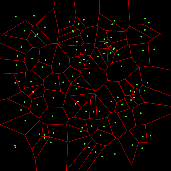
There is a little problem with some edges for cells on the border of the image: they are not drawn. That is because they are infinite.
Worse, a cell might not be in one piece. For instance, if we take three points aligned, the middle point will have two infinite half-edges not linked together. It is not very satisfactory because that means we cannot access to one of the half-edges as a cell is a linked list of edges.
To solve these problems, we will bound the diagram. By bounding the diagram, I mean that we will bound every cell of the diagram so that there are no infinite edges anymore and every cell is a closed polygon.
Fortunately, Fortune’s algorithm gives us a way to quickly find the infinite edges: they correspond to the half-edges still in the beachline at the end of the algorithm.
My bounding algorithm takes a box as input and has three steps:
- It will make sure that every vertices of the diagram is contained inside the box.
- Clip every infinite edge.
- Close the cells.
Step 1 is trivial, we just expand the box if it does not a contain a vertex.
Step 2 is pretty simple too, it just consists of computing intersections between rays and the box.
Step 3 is not very difficult neither, but it requires to be very careful. I do it in two steps. Firstly, I add the corners of the box to cells that need them in their vertices. Secondly, I make sure that all the vertices of a cell are linked by half-edges.
I encourage you to read the code or ask questions if you want more details on this part.
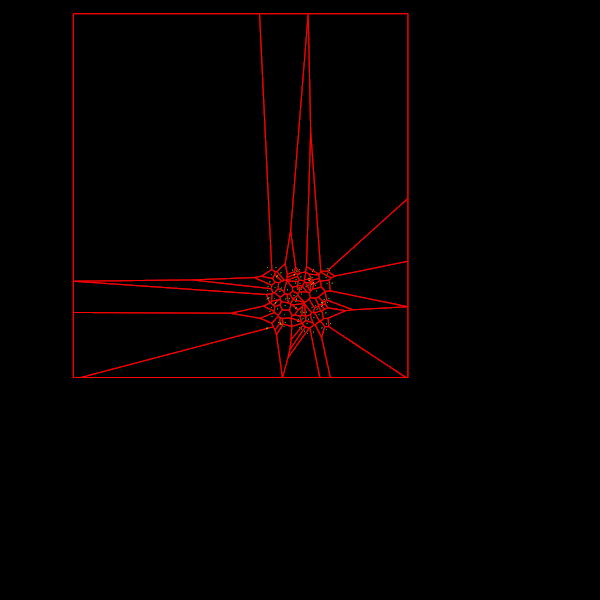
Here is the diagram output by the bounding algorithm:

We can see that all the edges are drawn now. And if we zoom out, we can check that all the cells are closed:
Intersection with a Box
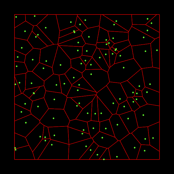
Cool! But the first image at the top of the article is cooler, isn’t it?
In many applications, it is useful to have the intersection between a Voronoi diagram and a box, it is what is shown on the first image.
The good news is that it is a lot easier now that we have bounded the diagram. The bad news is that once again even if the algorithm is not over-complicated, we will have to be careful.
The idea is the following: for each cell we traverse its half-edges and we check the intersection between this half-edge and the box. There are five cases:
- The half-edge is completely inside the box: we keep this half-edge
- The half-edge is completely outside the box: we discard this half-edge
- The half-edge is going outside the box: we clip the half-edge and we store it as the last half-edge that went outside.
- The half-edge is going inside the box: we clip the half-edge and we add half-edges to link it with the last half-edge that went outside (we store it at case 3 or 5)
- The half-edge crosses the box twice: we clip the half-edge, we add half-edges to link it with the last half-edge that went outside, and we store it as the new last half-edge that went outside.
Uh, that’s a lot of cases. I made a picture to visualize them:

The orange polygon is the original cell while the red one is the clipped cell. The clipped half-edges are depicted in red. The green ones are the ones added to link the half-edges that are going inside the box with the ones that are going outside.
After we applied this algorithm to the bounded diagram, we have the expected result:
Conclusion
This article was pretty long. And I am sure that many things are still unclear. Nevertheless, I hope you find it useful. Do not hesitate to read the code if you want to see all the details and if you have any question you can ask them in the comment section below.
To finish this article and to be sure we have not done all of this for nothing I have measured the time it takes to compute the Voronoi diagram for different numbers of sites on my (cheap) laptop:
- \(n = 1000\): 2ms
- \(n = 10000\): 33ms
- \(n = 100000\): 450ms
- \(n = 1000000\): 6600ms
I have nothing to compare these durations with, but it seems blazing fast!
References
- Steven Fortune’s original paper
- Computational Geometry, 3rd edition by Mark de Berg, Otfried Cheong, Marc van Kreveld and Mark Overmars
- Fortunes Algorithm: An intuitive explanation on jacquesheunis.com
- Fortune’s algorithm and implementation on blog.ivank.net
- Introduction to Algorithms, 3rd edition by Thomas H. Cormen, Charles E. Leiserson, Ronald L. Rivest and Clifford Stein
If you are interested in my adventures during the development of Vagabond, you can follow me on Twitter.