pvigier's blog
computer science, programming and other ideas
Commit Graph Drawing Algorithms
This article is one chapter of my master thesis entitled “Design and implementation of a graphical user interface for git”. It describes the algorithm I designed to draw the commit graph in my own prototype git client called gitamine. I have adapted the content so that it fits better with this blog.
Drawing graphs is a very complex topic in general but here we want to draw a specific type of graphs: commit graphs. Commit graphs have several several pieces of information that simplify the problem. The most important ones are that the graph is directed and acyclic and that the commits have timestamps.
Moreover, among the many ways we can draw a directed acyclic graph some are more appropriate for commit graphs. Indeed, programmers manipulate the branches of the graph thus it will be more convenient for them if the representation allows to visualize them easily.
We will first study the different types of graph drawing algorithms used in other clients. Then, we will describe how to place the nodes so that the commit graph is nicely drawable. Finally, we will cover some optimizations done in gitamine to draw and browse the graph in real time.
Types of Commit Graph Drawing Algorithms
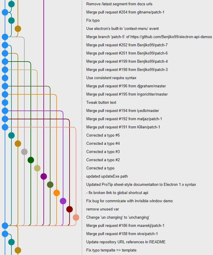
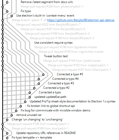
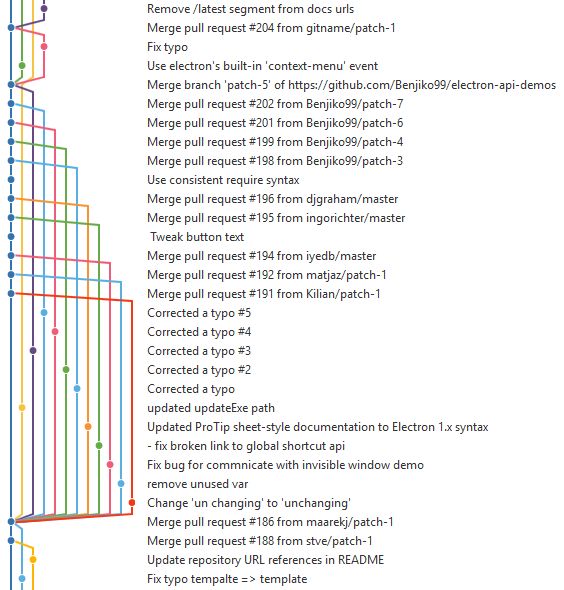
To start the study of commit graph drawing, we will look at how it is done by the other git clients. The figure below shows the same portion of a commit graph displayed by different git clients. This part was chosen because there are a lot of merges and we can clearly observe the differences between the graph drawing algorithms used by all the clients.
 |
 |
|---|---|
| Git Cola | Git Extensions |
 |
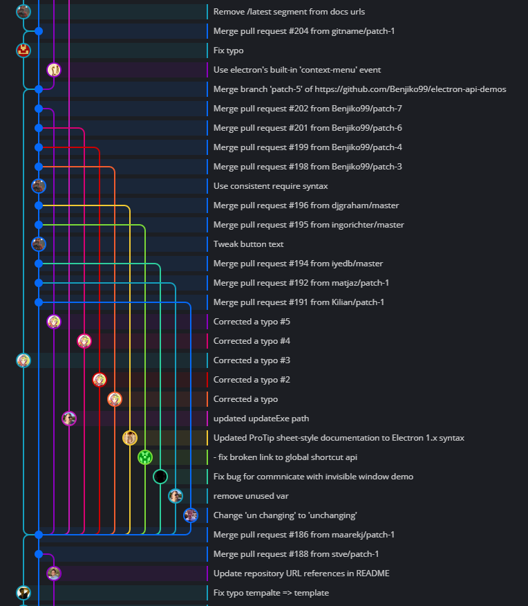 |
| gitk | GitKraken |
 |
 |
| SmartGit | SourceTree |
The first thing to observe is that there is no standard way to draw the commit graph. The different ways of drawing the commit graphs can be classified according to few design choices:
- one or several commits on the same row;
- straight branches i.e. all commits of the same branch are on the same column or curved branches.
We can see that Git Extensions and SmartGit seem to use a very similar algorithm with very curved branches. On the contrary, GitKraken draws branches as totally straight lines. SourceTree tries to keep branches as straight as possible but sometimes they curve. Git Cola’s algorithm has the particularity of placing several commits on the same row. The others draw the commit graph next to the commit history and thus they draw only one commit per row. Gitk draws a graph very similar to the one printed by the command git log --graph. It is much more compact than the other graphs because the commits have been reordered, the order does not follow the dates.
The table below sums up the characteristics of the graph drawing algorithms used by the clients.
| Client | One commit by row | Straight branches |
|---|---|---|
| Git Cola | No | No |
| Git Extensions | Yes | No |
| Gitk | Yes | No |
| GitKraken | Yes | Yes |
| SmartGit | Yes | No |
| SourceTree | Yes | No |
In gitamine, we will use an algorithm that draws only one commit by row to be able to show the commit graph and the commit history side-by-side as other git clients. Whether to draw straight or curved branches is a matter of taste. Personally, I found straight branches much more readable. Unfortunately, the only git clients that draw straight or almost straight branches, GitKraken and SourceTree, are not open-source, thus we will have to design our own algorithm.
Sorting Commits
In the two next sections, we will describe how to choose the position of the nodes so that the commit graph is drawable and readable. To simplify the problem, we will place the node on a 2D grid. We do not lose much in doing so because it is more pleasant to the human eye if the nodes are aligned.
In other words, we would like to find a function \(f\) from commits \(\mathcal{C}\) to \(\mathbb{N}^2\) which maps a commit \(c\) to its position on the grid \((i, j)\).
For the sake of simplicity, let us take the following notations for all commits \(c\) in \(\mathcal{C}\):
- \(c.parents\) is the ordered list of parents of \(c\).
- \(c.children\) is the unordered set of children of \(c\).
- \(c.i = f(c)_1\) is the \(i\)-coordinate associated to \(c\) by the function \(f\).
- \(c.j = f(c)_2\) is the \(j\)-coordinate associated to \(c\) by the function \(f\).
As said in the previous section, we would like to draw one commit by row. But we would also like to have all the edges, which are directed following the same direction. Without loss of generality, we choose that edges should go upward that is from a row \(i_1\) to a row \(i_2\) with \(i_1 > i_2\). To do that, we need that the parents of a commit are below this commit, namely f should respect the following condition:
\[\forall c \in \mathcal{C}, \forall d \in c.parents, d.i > c.i\]An order of commits that fulfills this condition is said to be topological.
Sorting by Date
The snippet below shows the content of a commit. We can observe that it contains two different timestamps respectively 1543445903 +0100 and 1543522724 +0100. The first one is the author date i.e. the date when the commit was created. The second is the committer date, it corresponds to the date when the commit was last modified.
tree 1060af6e25ad2351db05b3ec3803b0b2f78777a0
parent 524c8211e5a68bead1d12723a5b326af49933991
author Pierre Vigier <pierre.vigier@ymail.com> 1543445903 +0100
committer Pierre Vigier <pierre.vigier@ymail.com> 1543522724 +0100

Rewrite Event, Arc and VoronoiDiagram
A first idea is to sort the commits by the author date. This will work for very simple repository but certain operations like rebase or cherrypick allow to put commits with older author date as children of commits with more recent author date. Hence, if we sort the commit from newest to oldest author date and set \(c.i\) to the index of \(c\) in the sorted list, we would break the topological condition.
The second idea is to sort the commits by committer date. This is appealing as latest modifications of the developers will be shown first. Moreover, this order should be topological in most cases as when an operation is done on a commit, its committer date is updated. Thus, when a branch with old commits, according to their author dates, is rebased, their committer dates are updated and thus they will be more recent than the committer dates of their parents.
However, nothing guarantees that all operations in git will satisfy this property. For instance, if commits of a repository are created on two different computers with non-synchronized clocks, problems may happen. In addition, it is possible to manually set the author date and the committer date of a commit. Thus, it is possible to attribute an older committer date to a commit than the ones of its parents. In this case, the order given by committer date will not satisfy the topological condition.
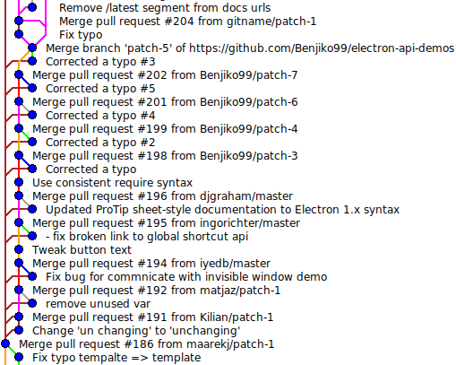
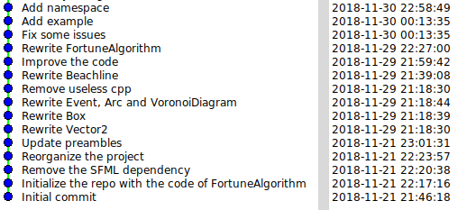
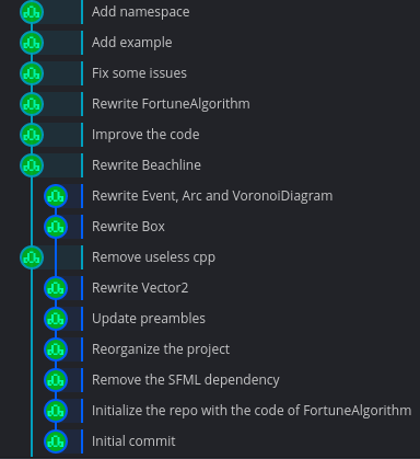
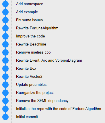
As a matter of fact, there exist repositories where the order according to committer dates is not a topological order. I suspect that GitKraken sorts the commits using committer date as it fails to draw correctly the graph on one of my repository as you can see in the figure below. The picture on the left shows the same repository displayed by a version of gitk modified to show the committer date in the right column instead of the author date. We can see that the commit with message “Remove useless cpp” has a committer date older than its parent.
 |
 |
|---|---|
| gitk | GitKraken |
Topological Sorting
The standard way to obtain an ordering of nodes of a directed acyclic graph that respects the condition given above is to do a topological sort.
The pseudo-code below is inspired from the section 22.4 of Introduction to Algorithms:
procedure topological_sort(C)
    function dfs(c)
        if not c.explored
            c.explored = true
            for d in c.children
                dfs(d)
            c.i = i
            i = i + 1

    i = 0
    for c in C
        dfs(c)
The idea is to use depth-first search to first explore and assign the \(i\)-coordinate of all the descendants of a commit before setting the one of this commit.
If we use a topological sort to order the commits, we are guaranteed that the graph can be drawn with all the edges going upward. However, the algorithm does not take the dates into account. Consequently, the last updates will not necessarily be at the top of the graph and could potentially be anywhere if the topology allows it which may not be natural to programmers.
Moreover, there may be many valid topological orders for a commit graph and the algorithm above will output one. But as there is no assumption on the order on which the commits in \(\mathcal{C}\) will be traversed there is no guarantee that the algorithm will always output the same topological order.
Temporal Topological Sorting
To solve the issues raised in the previous section, I slightly modified the algorithm so that the commits of \(\mathcal{C}\) are traversed according to their committer dates from newest to oldest:
procedure temporal_topological_sort(C)
    function dfs(c)
        if not c.explored
            c.explored = true
            for d in c.children
                dfs(d)
            c.i = i
            i = i + 1

    i = 0
    for c in C sorted from newest committer date to oldest
        dfs(c)
I called this algorithm temporal topological sort because it takes into account the topology of the graph and the timestamps of commits.
I would like to highlight the good properties of this algorithm:
- It outputs a topological order of the commits.
- The output is guaranteed to always be the same regardless of the order of commits in \(\mathcal{C}\).
- If there are no anomaly on committer dates, that is if the order induced by committer dates is already a valid topological order then the algorithm will return this order.
- It is blazing fast: its time complexity is \(O(n\log(n) + m)\) where \(n\) is the number of commits and \(m\) the number of edges.
Placing Commits
In the previous section, we have seen how to determine the \(i\)-coordinate of a commit. In other words, we have shown how to compute an order of the commits so that the edges can be drawn upward. In this section, we will see strategies to determine the \(j\)-coordinate of a commit.
Before getting to the heart of the matter, we must introduce some definitions that will simplify the discussion. We will separate the children of a commit in two categories: branch children and merge children.
A branch child is a child that continues a branch or creates a new one. While a merge child is a child that ends a branch by merging it into another one.
We can determine if a child is a branch child or a merge child of \(c\) by using the position of \(c\) in the list of parents of the child. The two following definitions formalize that.
For all \(c \in \mathcal{C}\), branch children of \(c\) are defined by: \(c.branchChildren = \{d \in c.children\text{ s.t. }d.parents[0] = c\}\)
For all \(c \in \mathcal{C}\), merge children of \(c\) are defined by: \(c.mergeChildren = \{d \in c.children\text{ s.t. }d.parents[0] \neq c\}\)
Curved Branches
The first algorithm we will describe is a simplistic method that works well for graph drawn with curved branches.
The idea is to maintain a list of active branches. Initially the list is empty, then we iterate the commits one by one from the lowest \(i\)-coordinate to the largest to find its position:
procedure curved_branches(C)
    Initialize an empty list of active branches B
    for c in C from lowest i-coordinate to largest
        if c.branchChildren is not empty
            select d in c.branchChildren
            replace d by c in B
        else
            insert c in B
        for d' in c.branchChildren \ {d}
            remove d' from B
        c.j = index of c in B
Let us make few remarks on the algorithm:
- A commit can only replace one of its branch children because they are the ones that extend the branch.
- We remove all the remaining branch children of \(c\) since they could only be replaced by \(c\), which is their first parent, but \(c\) replaces another commit.
The git clients that draw graphs with curved branches should use a very similar algorithm. However, there are two points that are still ambiguous:
- A commit may have several branch children. A strategy is to select the leftmost one i.e. the one with lowest \(j\)-coordinate.
- We do not precise where to insert \(c\) in the list of active branches. The simplest solution is to append.
We do not give more details for this version as we will do for the one with straight branches.
Straight Branches
In this section, we will describe an algorithm to draw the commit graph with straight branches i.e. with all the commits of a same branch on the same column. The advantage of this design is that it is easier to visualize branches which are a core concept of git.
Types of Edges
Firstly, let us make a distinction between two types of edges that will be represented differently as depicted in the figure below:
- edges between a commit and one of its branch children;
- edges between a commit and one of its merge children.
 |
 |
|---|---|
| Edge to branch children | Edge to merge children |
Algorithm
Secondly, let us describe a pseudo-code of the algorithm used to determine the \(j\)-coordinate of commits:
procedure straight_branches(C)
    Initialize an empty list of active branches B
    for c in C from lowest i-coordinate to largest
        compute forbidden j-coordinates J(c)
        if {d in c.branchChildren s.t. d.j is not it J(c)} is not empty
            select d in {d in c.branchChildren s.t. d.j is not in J(c)}
            replace d by c in B
        else
            insert c in B
        for d' in c.branchChildren \ {d}
            B[d'.j] = nil
        c.j = index of c in B
The algorithm looks quite similar to the one described in the previous section as both used a list of active branches. However, the key difference are:
- We compute a set of forbidden columns. These columns correspond to \(j\)-coordinates where if we place \(c\) there then there will be problem to link \(c\) with some of its children. The edges would overlap other commits or branches. We will detail how to define and compute \(J(c)\) later.
- We can insert \(c\) at an index of \(B\) equals to
nilif one is available, otherwise we append. - Instead of removing an element from \(B\), we just set its index to
nil.
Previously, in algorithm curved_branches, we could remove a branch from the list of active branches or insert one in the middle of it which would shift branches respectively to the left or to the right all the branches to the left of the removed branch. Now, we remove a branch by setting its index to nil and we can only append branches. These operations cause no shift of other branches and that is the reason why the branches are straight.
Forbidden Indices
We will now see how to determine and compute the set of forbidden indices \(J(c)\) for a commit \(c\). To do that, we will take a look at the example below.

We would like to compute the \(j\)-coordinate of the commit \(g\) which is the second parent of \(b\). So we need to draw an edge between a parent and a merge child. The list of active branches \(B\) is equal to \([f, nil, b, nil, c]\). We could insert at index \(1\) and \(3\) as these indices are equal to nil or append.
Let us examine the three cases:
- Index \(1\): the edge from \(g\) to \(b\) would overlap the commit \(e\).
- Index \(3\): the edge from \(g\) to \(b\) would overlap the edge from \(c\) to \(b\).
- Append: this index has never been used (as otherwise, it would be equal to
nil) so there cannot be any overlap.
Thus the right choice is to append \(g\) to \(B\), this results in the graph shown in the figure below.

We have shown that we must be careful when we process a commit that has merge children. In particular, we must be sure that there is no obstacle that prevents from linking the commit to one of its merge children.
For a branch child, there is no such problem because the edge follows the same column as the one on which the child is. And there is no obstacle in this case since the child is present in the list of active branches and prevent other commits or edges from occupying this column.
Thus, we can now give a definition for the set \(J(c)\):
\[J(c) = \underset{d \in c.mergeChildren}{\cup}{\{j \text{ s.t. the column j is non-empty between rows }d.i\text{ and }c.i\}}\]In layman terms, \(J(c)\) is the set of indices of columns where if \(c\) would be placed there, it would be impossible to link it with one of its children.
We can simplify the expression of \(J(c)\) thanks to the following lemma.
Lemma: \(J(c) = \{j \text{ s.t. the column j is non-empty between rows }\underset{d \in c.mergeChildren}{\min}{d.i}\text{ and }c.i\}\)
Let \(J_i(c)\) be equal to \(\{j \text{ s.t. the column j is non-empty between rows }i\text{ and }c.i\}\) for all \(i\). Then:
\[ J(c) = \underset{d \in c.mergeChildren}{\cup}{J_{d.i}(c)} \]But if \(i' < i\) then \(J_i \subseteq J_{i'}\). So:
\[ J(c) = J_{i_{min}}(c)\text{ with }i_{min} = \underset{c.mergeChildren}{\min}{d.i} \]I developed two methods to compute \(J(c)\) quickly.
In the first one, we maintain the list of \(J_i(c)\) for all commits that still have parents. Then when we want to compute \(J(c)\) for a commit \(c\), we just have to compute \(i_{min}\) and to retrieve \(J_{i_{min}}(c)\) which is equal to \(J(c)\) according to the previous lemma.
The second method uses an interval tree as described in section 14.3 of Introduction to Algorithms which is a data structure that allows to quickly find all intervals that intersect a given interval. The idea, here, is to add an interval of rows with the column as associated data in the interval tree each time we add a commit or an edge. Then when we want to find the occupied columns between \(i_{min}\) and \(c.i\), we just have to query the intervals that overlap with \([i_{min}, c.i]\).
Both methods were implemented and benchmarked on a large repository to see which is the most efficient. The table below presents the result of this benchmark.
| Method | Mean (ms) | Standard deviation (ms) |
|---|---|---|
| List of \(J_i(c)\) | 274 | 59.0 |
| Interval tree | 482 | 27.9 |
The mean and standard deviation are computed on 10 measures. We can see that the first method is faster. It is the one currently used by gitamine.
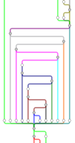
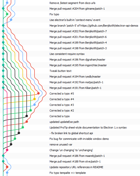
Finally, here are some examples of commit graphs drawn by gitamine:
|
 |
|---|---|
| Electron API Demos | MyGAL |
Optimizations
In the previous sections, we have shown how to compute the positions of each commits so that the graph is nicely drawable. In this section, we will discuss how to draw it effectively.
The first naive implementation allocates a canvas sufficiently large to draw the whole graph and draws it only once. However, for large repositories the canvas could be very large and use a lot of memory. The memory usage is in \(O(n \times w)\) where \(n\) is the number of commits and \(w\) is the width of the graph i.e the number of columns used. Thus, this implementation does not scale well in term of memory. Moreover, HTML canvasses are often implemented using GPU rendering and video memory is scarcer than main memory. In addition, Chromium seems to not manage well such big canvas. Indeed when scrolling, the application suffers important slowdowns.
Thus, the next step was to only allocate a canvas as large as the visible area. This method does not suffer from the problem described previously. However, we need to redraw each time the user scrolls or resizes the windows as the visible part of the graph changes.
To speed up the rendering, we need to render only what is actually visible. Finding the nodes that are visible is easy and can be done in constant time. We just have to find the first and the last commits visible by doing integer divisions of the top and bottom coordinates of the visible area by the height of a row.
However, determining the edges that are visible is more difficult. Indeed, edges that are linked to a visible commit are visible, but there may be edges that connect commits on both sides of the visible area as depicted in the figure below.

To find them quickly, we must recognize that this is a problem of finding intersecting intervals again. Indeed, we can represent all the edges by intervals of rows and the visible area is also an interval of rows. An edge is visible if and only if its interval overlaps with the interval of the visible area. So we can use an interval tree to find all the visible edges in \(O(k\log{m})\) where \(m\) is the number edges and \(k\) the number of edges that are visible.
In the table below, we can observe the time it takes to render the visible part of a large commit graph with and without the different optimizations we talked about:
| Method | Mean (ms) | Standard deviation (ms) |
|---|---|---|
| All nodes and all edges | 106 | 7.42 |
| Only visible commits but all edges | 26.8 | 3.37 |
| Only visible commits and edges | 0.580 | 0.606 |
The mean and the standard deviation are computed over 100 measures.
The last optimization does not concern the graph rendering but the commit list which is displayed next to the graph. Displaying the whole list of commits does not scale well when there are thousands or tens of thousands commits. Thus, we can apply the same idea as previously and only display the commits that are visible. However, to give the impression to the user that all the commits are displayed and give him the ability to scroll, padding was added before and after the displayed items.
If you are interested in my adventures during the development of Vagabond, you can follow me on Twitter.