Pychain Part 2 - Application: MNIST

13 Aug 2017 by pierre

In part 1, we have created a fully functional library which is able to create and train neural networks using computational graphs. We used them on very simple examples. Today, we are going to try it on a more serious problem: character recognition.

We are going to use a well-known database in the machine learning and deep learning world named MNIST. The database is available on Yann LeCun’s website. If you have read a bit about neural networks before you should have already seen his name. He is a French scientist who is one of the pioneers of neural networks and inventors of convolutional neural networks and he is now the director of AI at Facebook.

Character recognition is an emblematic problem for two reasons. Firstly, it is one of the first successes and industrial applications of neural networks. It was used since the 90’s to read checks. Secondly, computer vision has always been a leading application domain for neural networks.

In this part, we are going to briefly discover the MNIST database. Then, we are going to train some networks on it and finally, we are going to explore a bit how a neural network works.

MNIST Database

Get the Dataset

Firstly, you should download the four files named “train-images-idx3-ubyte.gz”, “train-labels-idx1-ubyte.gz”, “t10k-images-idx3-ubyte.gz”, “t10k-labels-idx1-ubyte.gz”. Then create a folder examples/mnist/mnist and uncompress them in the latter. If you have not already a file archiver, I can advise you to use 7-zip for Windows and The Unarchiver for MacOS. As for Linux users, you should already have one.

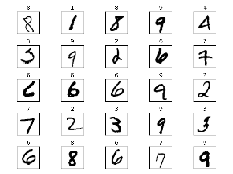
You can read the full specification on the database page. But it is not necessary, I have already written a script to read the database for you. You should only know that the database is separated on two parts: the training set and the test set. The training set contains 60 000 labelled images and we are going to use it to train the network. The test set contains only 10 000 labelled images and we are going to use it only to test the network, not to train it. It is very important to keep separated the two parts otherwise, your accuracy would be largely overestimated.

Preprocessings

Firstly, before training our computational graphs, we should preprocess the data. In general, a good thing to do is to center the data. To be clear, if we have \(x^{(1)}, ..., x^{(N)} \in \mathbb{R}^n\) as data, the centered vectors are defined by:

with \(\mu_j = \frac{1}{N}\sum_{i=1}^{N}{x^{(i)}_j}\).

Consequently, each dimension has its values centered around zero.

The other common preprocessing is to apply PCA. PCA gives an orthonormal basis in which the dimensions are decorrelated. If we note \(V\) the matrix which transforms the standard basis to this orthonormal basis. The new input vectors are:

We left multiply because we have adopted a row convention.

Finally, the last common preprocessing is to equalize the covariance. For doing this, we divide each dimension by its standard deviation:

with \(\sigma_j^2 = \frac{1}{N}\sum_{i=1}^{N}{(x^{(i)}_{d_j})^2}\).

Dividing by the standard deviation scales the values so that their order of magnitude is about 1.

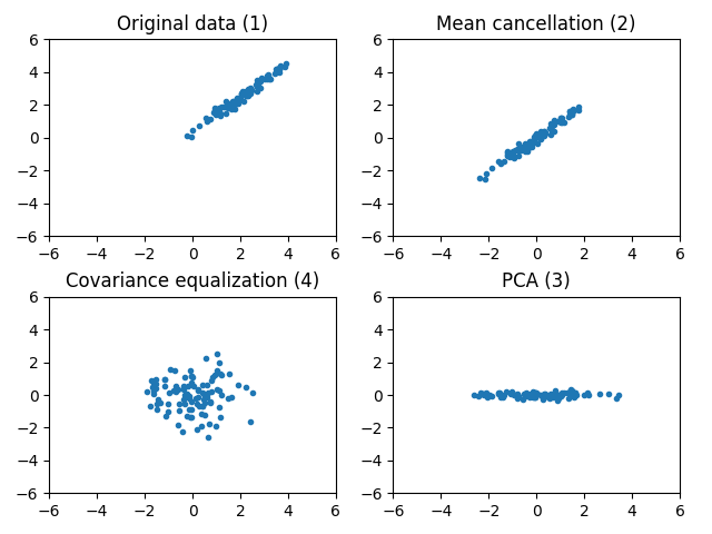
On the image below, you can see the effects of these three preprocessings. Notice the different effects of each of them.

You might ask why it is useful to preprocess the data before training. I think there are at least two reasons.

The first one is as there is no dominant or privileged dimension in the data, it can speed up the training. I think it is not totally obvious to see how the shape of the dataset can modify the shape of the cost function and help the gradient descent algorithm. So, I made a little simulation. I created a very simple dataset where the inputs have only one dimension with a mean of 2 and a standard deviation of 3. The outputs are given by \(f : x \mapsto 3x + 1\). Then I chose a very simple model, the linear regression, with only two parameters so that we can easily visualize the cost function. Finally, I chose the mean squared error as cost function.

Above, you can see that the shapes of the cost functions are very different. There is a dominant direction when the data are not preprocessed. Then you can see on the animation, the effect of the presence of a dominant direction on gradient descent. The algorithm tends to oscillate and does not go directly to the minimum.

If you want to see the code for the preprocessings and the animation of gradient descent, you can find it here.

The other advantage, is that when the data are normalized, it is easier to compare the parameters and the results with other problems. Many of the thumb rules for setting the hyperparameters such as the learning rates assume that the data are preprocessed.

In our case, we won’t use all these fancy things. We will keep things simple and only cancel the mean and divide by 255 to have the values in \([-0.5, 0.5]\). A reason why we don’t divide by the standard deviation is that some pixels are white in all the images and consequently their standard deviation is equal to zero.

def preprocess_dataset(X, mean=None):
    mean_X = np.mean(X, axis=0) if mean is None else mean
    return (X - mean_X) / 255, mean_X

In the function normalized_dataset, mean is an optional parameter because we want to compute the mean for the training set, but we want to apply the same preprocessings the test set.

Below, you can find all the steps to prepare the dataset.

# Prepare dataset
X, (nb_rows, nb_columns), Y = get_training_set('examples/mnist/mnist')
X, mean = preprocess_dataset(X)
X, Y = shuffle_dataset(X, Y)
Y = Y.reshape((len(Y), 1))
ohe_Y = one_hot_encode(Y)

X_test, (_, _), Y_test = get_test_set('examples/mnist/mnist')
X_test, _ = preprocess_dataset(X_test, mean)
X_test, Y_test = shuffle_dataset(X_test, Y_test)
Y_test = Y_test.reshape((len(Y_test), 1))

First, we retrieve the images thanks to the functions in mnist.py. Then we preprocess the dataset and shuffle it. Finally for the training, we create a one-hot encoded matrix for the labels called ohe_Y.

Our neural network won’t output a class directly. Instead it will output the probability distribution \(p(y \mid x)\) where \(x\) is the input. Concretely, for MNIST, the network will output a vector of \(\mathbb{R}^{10}\) which represents \((p(y=0 \mid x), \ldots, p(y=9 \mid x))\). So the network will learn to map an input to a distribution probability. Thus, our target outputs should also be a distribution probability. Consequently, we transform \(y^{(i)}\) to \(y^{(i)}_{ohe}\) according to:

(with the convention that the \(0^{th}\) element is the first one)

For instance, \(3\) will be mapped to \((0, 0, 0, 1, 0, 0, 0, 0, 0, 0)\) and \(9\) to \((0, 0, 0, 0, 0, 0, 0, 0, 0, 1)\).

That’s all for the dataset and preprocessings. We are now ready to train some neural networks!

Training

Let’s start by creating a very simple network with only one layer of 10 neurons.

# Create the graph
layers = [10]
batch_size = 128
learning_rate = 1
nb_times_dataset = 1
graph = create_fully_connected_network(layers)

The function create_fully_connected_network is very similar to the one of the previous part. I didn’t paste the code, you can retrieve it there in examples/mnist. But I add a little diagram to visualize what the function is doing:

As you can see, the function creates a multilayer network where the hidden layers use \(\tanh\) as activation function and the output layer uses \(softmax\) to create a distribution probability. Finally, the cost function is included in the graph and it is a categorical cross entropy. You can learn more about the output functions and cost functions in the corresponding appendix.

The function train_and_monitor train the graph, it is also similar to the code of the previous part but a little more complete.

def train_and_monitor(monitor=True):
    start_time = time.time()
    t = []
    accuracies_training = []
    accuracies_test = []
    i_batch = 0
    # Optimization algorithm
    sgd = GradientDescent(graph.get_parameter_nodes(), learning_rate)
    for i in range(nb_times_dataset):
        for j in range(0, X.shape[0], batch_size):
            # Train
            graph.propagate([X[j:j+batch_size]])
            cost = graph.backpropagate([ohe_Y[j:j+batch_size]])
            sgd.optimize(batch_size)
            # Monitor
            i_batch += 1
            print('pass: {}/{}, batch: {}/{}, cost: {}'.format(i, nb_times_dataset, \
                    j // batch_size, X.shape[0] // batch_size, cost / batch_size))
            if monitor and (i_batch % 256) == 1:
                t.append(i_batch)
                accuracies_training.append(accuracy(graph, X, Y))
                accuracies_test.append(accuracy(graph, X_test, Y_test))

There is a parameter monitor which allows to enable monitoring. If it is activated, the accuracy on the training and the test set will be computed periodically. Then at the end of the training, the learning curves will be shown. It is very practical to analyze the dynamic of training or to check if overfitting occurred.

All that remains to do is calling the function! With this architecture, you should obtain about 91.5% of accuracy with only one pass over the dataset and reach more than 92% with more passes. One pass takes a little less than 3s on my computer. I find the performance pretty decent!

To modify the architecture, you just have to change the value of the variable layer. For instance, to use a 3 layers neural network whose layers have respectively a size of 128, 64 and 10, you just have to replace layers = [10] by layers = [128, 64, 10]. After 10 passes, these architectures achieve 97.8% of accuracy. It is an incredible result for our little library!

Interpretation

Our networks achieve great results, but can we go further and try to understand a bit how they work? We will explore two ways of understanding them. Firstly, we are going to try to understand the role of the weights and we will conjecture that neural networks combine elementary features to create complex ones and finally take a decision. Then, we will see that indeed, neural networks create features that are discriminating and allows to take a decision.

Weights

The first layer of neurons directly takes the intensities of pixels as inputs. Consequently, it is possible to visualize the weights and to interpret them.

If \(W\) is the weights matrix of the first layer which contains \(m\) neurons then the \(j^{th}\) column corresponds to the \(j^{th}\) neuron and the coefficient \(w_{ij}\) to the weight of neuron \(j\) associated to pixel \(i\). Thus, it is possible to reshape the \(j^{th}\) column into an image and see the importance of each pixel for each neuron. The image below shows clearly how to interpret the weights matrix:

If we take a one layer neural network, there are 10 neurons which corresponds respectively to the digits 0, 1, …, 9. So the first neuron must find weights that determines well what is a zero, the second what is a one, …

Let’s call the function display_weights which reshape the weights and plot them see to check our hypothesis:

Very cool! We can clearly see that the weights of each neuron represent a sort of pattern of each digit. The network learns the discriminating shapes and parts of each digits.

Now what happens for a multilayer network? When they are several layers the neurons of the first layer do not correspond to any digit. Their outputs are used by the next layers and it is the neurons of the last layer which correspond to specific digits.

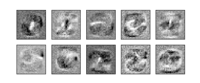
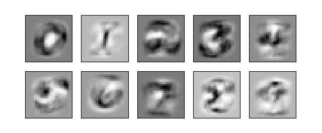
Let’s see the weights of the first layer of a multilayer network [64, 32, 16, 10]:

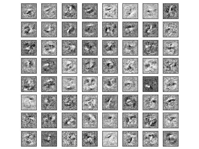
It is way more difficult to see digits in the weights. However, we can see small areas which are really bright of dark. These small areas correspond to small shapes which are discriminating.

For example, on the image of the 5th row and 7th column we can see a bright area which is looking for the presence of black pixels there. This neuron will output a positive value for digits where these pixels are black. This is the case for 8 and 6. On the contrary, It will output negative values for a 3 or a 9. Consequently, it allows to discriminate the digits with a closed loop at the bottom and those which have not got one.

The next layers will then combine these basic features to create more complex ones. And finally, the last layer will take these deep features created by the first layers as input to take the final decision.

Deep Features

Let’s look a bit more at these deep features.

A multilayer neural network can be divided in two parts. The first layers which create the deep features and the last layer which gives the output. However, it is important to remark that the last layer is simply a linear classifier.

The linear classifiers are really simple to analyze and understand. We will consequently study them in order to understand a bit more the deep features.

Linear Classifiers

We will describe two types of linear classifier: the binary linear classifier and the multiclass linear classifier.

The output of a binary linear classifier is a single real number given by:

Then the chosen class is \(g(x) = \left\{\begin{array}{rl}1 & \text{ if } f(x) \geq 0.5 \\ 0 & otherwise \end{array}\right.\).

And the output of multiclass is a probability distribution stored in a vector where the \(k^{th}\) coordinate is given by:

Then the chosen class is \(g(x) = \underset{k}{argmax}(f(x)_k)\).

By the way they are called linear classifiers because they use linear combinations of the input to compute the output.

What it is interesting to know for a classifier is the shape of its frontiers. Let \(A_k = \{ x \in \mathcal{X}, g(x) = k \}\), it is the subset of the input space for which the output class is \(k\), we will call \(A_k\) the decision area for class \(k\). The frontiers are the areas which separate an \(A_i\) from another \(A_j\).

Let’s determine the decision areas and the frontiers. In order to do that, I have written a small program which randomly creates a linear classifier and plots the decision areas. You can get it here. Here are the results for a binary classifier and a multiclass classifier:

Binary	Multiclass

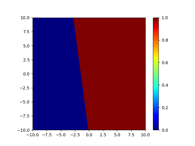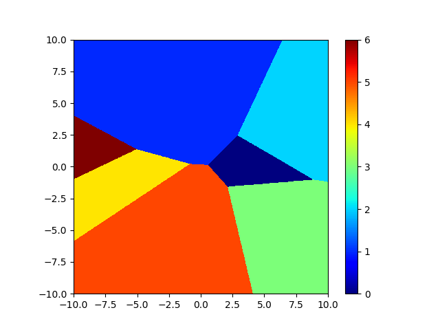For a binary linear classifier, the input space is divided in two half-spaces by a hyperplane, which is a line in 2D.

For a multiclass linear classifier, the input space is divided in cells which are intersection of half-spaces. Concretely, the cells have their sides which are flat.

If you want to formally prove these results, you can look at the exercises at the end of this part.

What we have seen is that if we want a linear classifier to correctly classify our inputs, it should be possible to separate the different classes with hyperplanes. We often say that the classes should be linearly separable

Generally, the classes are not linearly separable so the accuracy of linear classifiers is not great. That’s a reason why we use neural networks to create non-linear functions which are able to model non-linear frontiers.

This is a point of view, now we can see another one. Multilayer neural networks try to find a transformation from the input space \(\mathcal{X}\) where the classes are not linearly separable to a space of deep features where they are.

In the next parts, we will show several examples where neural networks are indeed able to create deep features that make classes linearly separable or almost.

Deep Features in XOR and the Disk

Do you remember the two examples of the previous part? They were very simple problems where the frontiers were non-linear. Hence, they are perfect candidates to see if the deep features are linearly separable.

I have slightly modified the code which creates the computational graph in order to have access to the output of the last layer.

In addition, I have added the function display_deep_features which displays the deep features. I copy the code below:

def display_deep_features(graph, X, Y):
    plt.figure()
    # Compute the deep features
    features = graph.propagate([X])[1]
    # PCA with 2 components
    features -= np.mean(features, axis=0)
    U, S, V = np.linalg.svd(features)
    points = np.dot(features, V.T[:,:2])
    # Plot points for each digit
    for i in range(2):
        x, y = points[Y == i,:].T
        plt.plot(x, y, 'o', label=str(i))
    plt.legend()
    plt.title('Deep features')

It computes the deep features for at most 1000 points. Note that we select the second output of the graph with [1] which is the output of the penultimate layer.

Then it applies PCA to project the deep features into the 2D space. The deep features space could have a high dimension so we must project them in 2D to be able to visualize them. Recall that PCA finds a good subspace in which to project to loss the minimum of information.

Finally, we plot the projected deep features.

Here are the results for XOR:

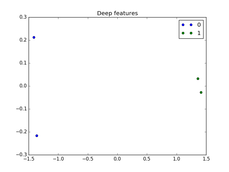
The four points of the dataset which were not linearly separable now clearly are.

And here are two different results for the disk problem:

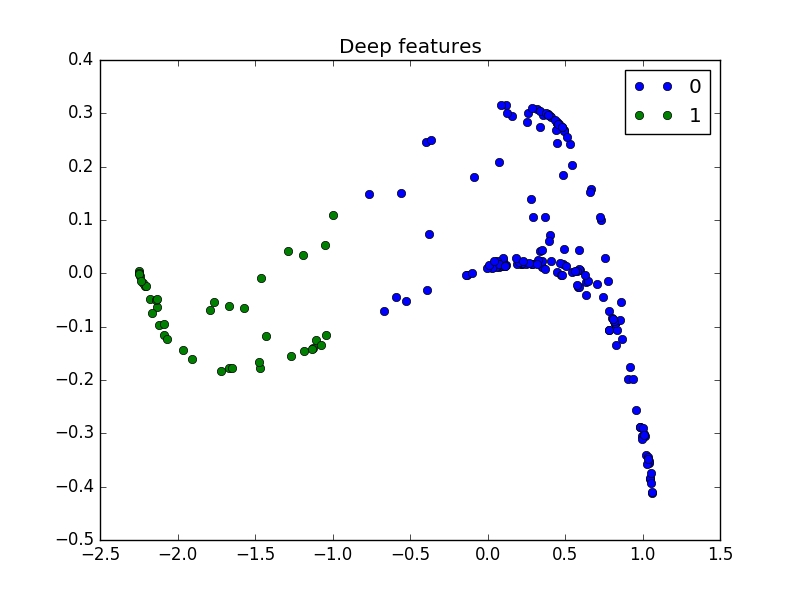
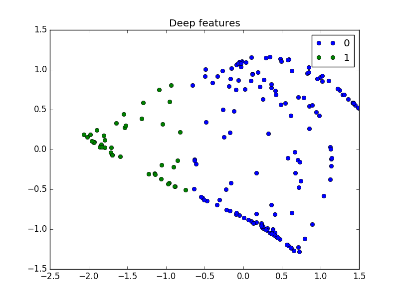
These are great figures! In both cases, the deep features make the dataset linearly separable.

On these simple problems, neural networks successfully transform the inputs to deep features where classes are linearly separable.

Deep Features in MNIST

Let’s do the same experiment on MNIST. I use the network [128, 64, 10] which gives very good accuracy and I obtain this result:

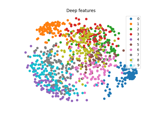
The points of a same color are clearly gathered on a same region of the space, but it is clearly not linearly separable.

The first explanation is that the network does not obtain an accuracy of 100% but only 97.8% so the deep features should only be almost linearly separable. However, this does not completely explain this messy result.

The other explanation is that the deep features are almost linearly separable in their space which has here 64 dimensions. And when we project the deep features in 2D we totally loose the linear separability.

Let’s try to project them in the 3D space in order to retain more information:

That’s a lot better. The classes are more separated in the space.

Conclusion

I hope that you earn a bit of intuition on neural networks through these experiments.

To conclude this part, I am going to sum up the different results we have seen:

• The first layer of a multilayer neural network creates basic features from the data which are then combined by other layers to create more complex features.
• A neural network can be divided in two parts: a part which create deep features and another part which is a linear classifier and uses the deep features to give an output.
• During training, a neural network looks for a good transformation which makes the deep features of the dataset linearly separable.

To Go Further

Some problems to have fun:

• Try to find the best architecture and parameters to achieve the highest accuracy on the test set. Clues

• The shape in the weights are a bit noisy. Add weight decay in the model and see how it smoothes the shapes. Explain the phenomenon. Clues

• Proof that a binary linear classifier separates the space in two half-spaces and that a multiclass linear classifier separates the space in cells which are intersection of half-spaces. Clues

If you are interested in my adventures during the development of Vagabond, you can follow me on Twitter.

Tags: math python